Part 1. Introduction
NLP Tutorial
Part 1: Introduction
Supervised Learning Paradigm
Supervised Learning: Where the ground truth for targets can be found in observations.
Observations: Items we want to predict from. Denoted with x value or called input
Targets: Labels that correspond to an observation. Denoted with x value or called ground truth
Model: Function that takes obervations to predict targets
Parameter: Weights of observations to parameterize model. Denoted with w
Predictions: Estimates of targets for observations. Denoted with y hat or ŷ
Loss Function: Calculates how far the predictions are from the ground truth and gives a real scalar value, loss. Denoted with L
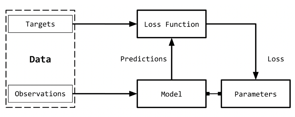
For an input X, the model F is ŷ = F(X, w) and the loss function L is L(y,ŷ)
Gradient Descent is commonly used to find the roots of a linear system. w is iteratively updated over all of x until L reaches a certain threshold.
An alternative to this is Stochastic Gradient Descent which uses random numbers or random “minibatches” instead of random numbers.
Iteratively updating parameters of the model is known as Backpropagation. The forward step is used to calculate the Loss and the backward step is used to update the parameters.
Observation and Target Encoding

Text can be represented as a numerical vector which is also a count-based representation based on heuristics.
One-Hot Representation
Starts with a zero vector and sets 1 to the corresponding index of the word if present in the text.
Ex:
This is the best day ever.
This is the best laptop here.
Vocabulary: {‘this’, ‘is’, ‘the’, ‘best’, ‘day’, ‘laptop’, ‘ever’, ‘here’}
Binary encoding for “this is the best” is [1,1,1,1,0,0,0,0]
| this | is | the | best | day | laptop | ever | here | |
|---|---|---|---|---|---|---|---|---|
| 1this | 1 | 0 | 0 | 0 | 0 | 0 | 0 | 0 |
| 1is | 0 | 1 | 0 | 0 | 0 | 0 | 0 | 0 |
| 1the | 0 | 0 | 1 | 0 | 0 | 0 | 0 | 0 |
| 1best | 0 | 0 | 0 | 1 | 0 | 0 | 0 | 0 |
| 1day | 0 | 0 | 0 | 0 | 1 | 0 | 0 | 0 |
| 1laptop | 0 | 0 | 0 | 0 | 0 | 1 | 0 | 0 |
| 1ever | 0 | 0 | 0 | 0 | 0 | 0 | 1 | 0 |
| 1here | 0 | 0 | 0 | 0 | 0 | 0 | 0 | 1 |
One-hot representation for encoding the sentences “This is the best day ever” and “This is the best laptop here”
TF Representation
TF Representation is the sum of one-hot representations of each word in the sentence. The sentence “This here is the best laptop this day” using the previous one-hot encoding would give the encoding [2, 1, 1, 1, 1, 1, 0, 1].
from sklearn.feature_extraction.text import CountVectorizer
import seaborn as sns

corpus = ["This is the best day ever", "This is the best best laptop here"]
vocab = {'this', 'is' ,'the','best', 'day' ,'laptop', 'ever', 'here'}

one_hot_vectorizer = CountVectorizer(binary=True)
one_hot = one_hot_vectorizer.fit_transform(corpus).toarray()
sns.heatmap(one_hot, annot=True, cbar=False, xticklabels=vocab, yticklabels=['Sentence 1','Sentence 2'])
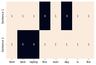
Collapsed one-hot representation with the corpus “This is the best day ever” and “This is the best best laptop here”.
TF-IDF Representation
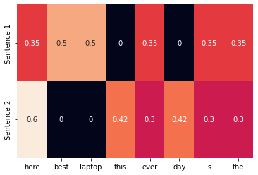
The TF-IDF representation uses the word’s frequency in the corpus to weight said words. Common words are not as important but the rarer words will have more weight.
The Inverse Document Frequency (IDF) is the log of the number of documents divided by the number of documents containing the word.
from sklearn.feature_extraction.text import TfidfVectorizer
import seaborn as sns

tfidf_vectorizer = TfidfVectorizer()
tfidf = tfidf_vectorizer.fit_transform(corpus).toarray()
sns.heatmap(tfidf, annot=True, cbar=False, xticklabels=vocab, yticklabels= ['Sentence 1', 'Sentence 2'])
Target Encoding
Most NLP tasks use unique categorical labels but that can have issues as output labels increase such as in the language modeling problem which is to predict the next word. The label space will include everything from special characters, names, etc. so we must find a better solution for this.
Other NLP problems use labels use numerical labels but this can be easily satisfied by making “bins” or ranges for all of the values. (Ex: 0-20, 20-40, … , 180-200)
Computational Graphs
A computational graph is an abstraction which models math expressions. For our purposes, computational graphs will help us see what kind of additional differentiation is required to get parameter gradients
For a linear model, the equation used would be
y = wx + b
which can be simplified into
z = wx & y = z + b
A directed acyclic graph (DAG) of the aforementioned equations would look like so:

PyTorch Basics
We will be using PyTorch for this course. PyTorch is a tensor manipulation library that offers a multitude of deep learning packages.
A tensor is a mathmatical data structure wherein there is some dimensions of data. A Rank 0 Tensor has but one value, a Rank 1 Tensor is a vector, a Rank 2 Tensor is a matrix, and so on as the Rank N Tensor is an n-dimensional array of scalars.
Installing PyTorch
Download using either Pip or Conda
Use this command for installation using conda
conda install pytorch torchvision -c pytorch
Creating Tensors
Create a helper function display(x) so that we can see important attributes of the tensor easily.
import torch

def display(x):
    print("Tensor Type: {}".format(x.type()))
    print("Tensor Size: {}".format(x.shape))
    print("Values: \n{}".format(x))


display(torch.Tensor(3, 4))
Tensor Type: torch.FloatTensor
Tensor Size: torch.Size([3, 4])
Values:
tensor([[ 9.4774e-38,  2.2960e-38, -1.7292e-23,  4.5869e-41],
        [ 0.0000e+00,  1.0842e-19, -2.4786e+15, -1.0845e-19],
        [-1.7267e-23,  4.5869e-41, -1.5941e-24,  4.5869e-41]])
There’s a number of ways to randomly initialize a tensor’s values as well, either uniformly random and randomly from a normal distribution
display(torch.rand(2, 3))  # uniformly random
display(torch.randn(2, 3)) # random normal distribution
Tensor Type: torch.FloatTensor
Tensor Size: torch.Size([2, 3])
Values:
tensor([[0.9510, 0.5519, 0.4149],
        [0.5744, 0.3234, 0.8496]])
Tensor Type: torch.FloatTensor
Tensor Size: torch.Size([2, 3])
Values:
tensor([[ 0.9831,  0.1202, -0.3810],
        [-0.6465,  0.1269, -0.5633]])
Tensors can also be filled by one value or certain values. torch.zeros and torch.ones both fill up the tensor with the given dimensions with 0’s and 1’s respectively. torch.fill_ takes the given defined tensor, and fills up every value with the given value.
filledTensor = torch.zeros(2, 3) #Fills tensor with 0s
display(filledTensor)

filledTensor = torch.ones(2, 3) #Fills tensor with 1s
display(filledTensor)

filledTensor.fill_(8) #Fills tensor with 8s
display(filledTensor)
Tensor Type: torch.FloatTensor
Tensor Size: torch.Size([2, 3])
Values:
tensor([[0., 0., 0.],
        [0., 0., 0.]])
Tensor Type: torch.FloatTensor
Tensor Size: torch.Size([2, 3])
Values:
tensor([[1., 1., 1.],
        [1., 1., 1.]])
Tensor Type: torch.FloatTensor
Tensor Size: torch.Size([2, 3])
Values:
tensor([[8., 8., 8.],
        [8., 8., 8.]])
Tensors can also be defined by lists and by numpy arrays.
import numpy as np

listTensor = torch.Tensor([[1, 2, 3],
                           [4, 5, 6]])
display(listTensor)

numpyArray = np.random.rand(2, 3)
display(torch.from_numpy(numpyArray))
Tensor Type: torch.FloatTensor
Tensor Size: torch.Size([2, 3])
Values:
tensor([[1., 2., 3.],
        [4., 5., 6.]])
Tensor Type: torch.DoubleTensor
Tensor Size: torch.Size([2, 3])
Values:
tensor([[0.2463, 0.6978, 0.6044],
        [0.7769, 0.3949, 0.9071]], dtype=torch.float64)
Tensor Types and Size
Just like numerical values, Tensor’s can also vary in their types which include float (the default), long, double, etc.
This can be changed by calling the specific Tensor type’s constructor or through torch.tensor() and passing the wanted data type.
display(listTensor)

listTensor = listTensor.long()
display(listTensor)

listIntTensor = torch.tensor([[1, 2, 3],
                             [4, 5, 6]], dtype=torch.int64)
display(listIntTensor)

listIntTensor = listIntTensor.double()
display(listIntTensor)
Tensor Type: torch.FloatTensor
Tensor Size: torch.Size([2, 3])
Values:
tensor([[1., 2., 3.],
        [4., 5., 6.]])
Tensor Type: torch.LongTensor
Tensor Size: torch.Size([2, 3])
Values:
tensor([[1, 2, 3],
        [4, 5, 6]])
Tensor Type: torch.LongTensor
Tensor Size: torch.Size([2, 3])
Values:
tensor([[1, 2, 3],
        [4, 5, 6]])
Tensor Type: torch.DoubleTensor
Tensor Size: torch.Size([2, 3])
Values:
tensor([[1., 2., 3.],
        [4., 5., 6.]], dtype=torch.float64)
Tensor Operations
Just like many data structures, the +,-,/,* operations work as well as .add().
listTensor = torch.Tensor([[1, 2, 3],
                           [4, 5, 6]])
display(listTensor)

display(listTensor*3) # Multiply all values by 3

display(listTensor+listTensor) # Add it to itself

display(torch.add(listTensor,listTensor)) # Add it to itself using torch.add()

display(listTensor*listTensor) # Multiplies each value to the corresponding value (NOT matrix multiplication)
Tensor Type: torch.FloatTensor
Tensor Size: torch.Size([2, 3])
Values:
tensor([[1., 2., 3.],
        [4., 5., 6.]])
Tensor Type: torch.FloatTensor
Tensor Size: torch.Size([2, 3])
Values:
tensor([[ 3.,  6.,  9.],
        [12., 15., 18.]])
Tensor Type: torch.FloatTensor
Tensor Size: torch.Size([2, 3])
Values:
tensor([[ 2.,  4.,  6.],
        [ 8., 10., 12.]])
Tensor Type: torch.FloatTensor
Tensor Size: torch.Size([2, 3])
Values:
tensor([[ 2.,  4.,  6.],
        [ 8., 10., 12.]])
Tensor Type: torch.FloatTensor
Tensor Size: torch.Size([2, 3])
Values:
tensor([[ 1.,  4.,  9.],
        [16., 25., 36.]])
There are also a various number of ways to change and view Rank 2 tensors differently
tensorRankOne = torch.arange(6)
display(tensorRankOne)

tensorRankOne = tensorRankOne.view(2, 3) # rearrage it into a rank 2 tensor
display(tensorRankOne)

display(torch.sum(tensorRankOne, dim=0)) # get sum of each column
display(torch.sum(tensorRankOne, dim=1)) # get sum of each row

display(torch.transpose(tensorRankOne, 0, 1)) # swap the axis or transpose the tensor
Tensor Type: torch.LongTensor
Tensor Size: torch.Size([6])
Values:
tensor([0, 1, 2, 3, 4, 5])
Tensor Type: torch.LongTensor
Tensor Size: torch.Size([2, 3])
Values:
tensor([[0, 1, 2],
        [3, 4, 5]])
Tensor Type: torch.LongTensor
Tensor Size: torch.Size([3])
Values:
tensor([3, 5, 7])
Tensor Type: torch.LongTensor
Tensor Size: torch.Size([2])
Values:
tensor([ 3, 12])
Tensor Type: torch.LongTensor
Tensor Size: torch.Size([3, 2])
Values:
tensor([[0, 3],
        [1, 4],
        [2, 5]])
Indexing, Slicing, and Joining
Very similar to NumPy’s way of indexing and slicing. PyTorch also has it’s own functions for more complex indexing and slicing as well
tensorRankTwo = torch.arange(6).view(2,3)
display(tensorRankTwo)

display(tensorRankTwo[:1, :2])

display(tensorRankTwo[0, 1])

indices = torch.LongTensor([0, 2])
display(torch.index_select(tensorRankTwo, dim=1, index=indices)) # get the first and second column

indices = torch.LongTensor([0, 0, 0])
display(torch.index_select(tensorRankTwo, dim=0, index=indices)) # get the first row 3 times

display(torch.cat([tensorRankTwo,tensorRankTwo], dim=0)) # Concatenation of second tensor to the bottom of first tensor

display(torch.cat([tensorRankTwo,tensorRankTwo], dim=1)) # Concatenation of each row of the tensors
Tensor Type: torch.LongTensor
Tensor Size: torch.Size([2, 3])
Values:
tensor([[0, 1, 2],
        [3, 4, 5]])
Tensor Type: torch.LongTensor
Tensor Size: torch.Size([1, 2])
Values:
tensor([[0, 1]])
Tensor Type: torch.LongTensor
Tensor Size: torch.Size([])
Values:
1
Tensor Type: torch.LongTensor
Tensor Size: torch.Size([2, 2])
Values:
tensor([[0, 2],
        [3, 5]])
Tensor Type: torch.LongTensor
Tensor Size: torch.Size([3, 3])
Values:
tensor([[0, 1, 2],
        [0, 1, 2],
        [0, 1, 2]])
Tensor Type: torch.LongTensor
Tensor Size: torch.Size([4, 3])
Values:
tensor([[0, 1, 2],
        [3, 4, 5],
        [0, 1, 2],
        [3, 4, 5]])
Tensor Type: torch.LongTensor
Tensor Size: torch.Size([2, 6])
Values:
tensor([[0, 1, 2, 0, 1, 2],
        [3, 4, 5, 3, 4, 5]])
Tensors and Computational Graphs
While defining a Tensor, another action that can be done is tracking the tensor’s current gradient and gradient function. This can be done by
requires_gradient = true
gradientTensor = torch.ones(2, 2, requires_grad=True)

display(gradientTensor)
print(gradientTensor.grad is None)

changedTensor = (gradientTensor + 2) * (gradientTensor + 5) + 3
display(changedTensor)
print(gradientTensor.grad is None)

meanTensor = changedTensor.mean()
display(meanTensor)
meanTensor.backward()
print(gradientTensor.grad is None)
Tensor Type: torch.FloatTensor
Tensor Size: torch.Size([2, 2])
Values:
tensor([[1., 1.],
        [1., 1.]], requires_grad=True)
True
Tensor Type: torch.FloatTensor
Tensor Size: torch.Size([2, 2])
Values:
tensor([[21., 21.],
        [21., 21.]], grad_fn=<AddBackward0>)
True
Tensor Type: torch.FloatTensor
Tensor Size: torch.Size([])
Values:
21.0
False
By setting requires_grad=True , PyTorch now has to manage the gradient computation’s forward passes. Backward pass is initiated by .backward() which evaluates a loss function.
The gradient is typically is the slope of a function’s output with respect to its input. The nodes’ gradients can be accessed using the .grad for the respective member variable. Optimizers also use the .grad variable to update the parameters.
CUDA Tensors
Utilizing the GPU of your laptop allows for faster processing. Through the usage of the CUDA API, you can allocate the tensor to GPU memory on NVIDIA GPUs.
First you must check if CUDA can be supported, if so then create a torch device that utilizes the GPU and use .to(device) to instantiate future tensors to the GPU.
It is not possible to operate with CUDA and non-CUDA tensors not on the same device.
device = torch.device("cuda" if torch.cuda.is_available() else "cpu")
print(device)

cudaTensor = torch.rand(3, 3).to(device)
display(cudaTensor)
cpu
Tensor Type: torch.FloatTensor
Tensor Size: torch.Size([3, 3])
Values:
tensor([[0.2927, 0.6019, 0.4595],
        [0.0556, 0.1222, 0.7028],
        [0.1000, 0.7749, 0.7047]])
Enjoy Reading This Article?
Here are some more articles you might like to read next: