Part 3. Foundations of Neural Nets
NLP Tutorial
Part 3: Foundations of Neural Nets
The Perceptron: The Simplest Neural Network
Similarly modeled after the biological neuron, the perceptron has signals flowing from the input to output. Typically there is more than just one input so an equation modeling would have the weights (w), bias (b), and an activation function (f) in addition to the input (w), a vector, and the output (y).
y = f( w⋅x + b )
In most cases, f is a nonlinear function and the expression ‘w⋅x + b’ is a linear function meaning that a perceptron is composed of a nonlinear and a linear function. The linear expression can also be called an affine transform
Let’s create our own Perceptron object:
import torch
import torch.nn as nn

class Perceptron(nn.Module):
    """ A perceptron is one linear layer """
    def __init__(self, input_dim):
        """
        Args: input_dim (int): size of the input features
        """
        super(Perceptron, self).__init__()
        self.fc1 = nn.Linear(input_dim, 1)

    def forward(self, x_in):
        """The forward pass of the perceptron
        Args:
            x_in (torch.Tensor): an input data tensor
            x_in.shape should be (batch, num_features)
        Returns:
            the resulting tensor. tensor.shape should be (batch,).
        """
        return torch.sigmoid(self.fc1(x_in)).squeeze()
Activation Function
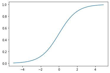
Sigmoid
Sigmoid: Earliest activation functions which takes a real number and brings it down to a value between 0 and 1
\[f(x) = \frac{1}{1+e^{-x}}\]By graphing the sigmoid function, we can see that its a differentiable function. However, there can be issues sometimes around zero and as x aproaches either infinity as the gradients becomes 0 or overflow. Due to this we only use the Sigmoid function as part of the output of a model.
import matplotlib.pyplot as plt

x = torch.arange(-5., 5., 0.1)
y = torch.sigmoid(x)
plt.plot(x.numpy(), y.numpy())
plt.show()
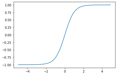
Tanh
\[f(x) = tanh x = \frac{e^x - e^{-x}}{e^x + e^{-x}}\]Having a similar shape to that of the Sigmoid, the gradients that it provides however vary much more as the minimum is -1 and the maximum is 1.
x = torch.arange(-5., 5., 0.1)
y = torch.tanh(x)
plt.plot(x.numpy(), y.numpy())
plt.show()
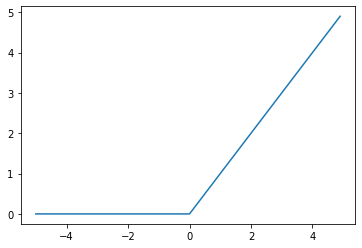
ReLU
ReLU: Rectified Linear Unit
One of the most commonly used activation functions in all of Deep Learning but it is quite simple. What it does is set all negative values to 0 and if the value is a real positive number, it stays that way.
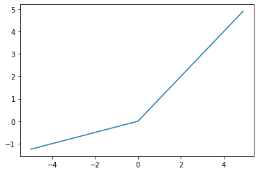
\[f(x) = max(0,x)\]However, somtimes the output becomes 0 and never recovers. To solve this there are slight variations to ReLU, namely Leaky ReLU and Parametric ReLU (PReLU).
print("ReLU")
relu = torch.nn.ReLU()
x = torch.arange(-5., 5., 0.1)
y = relu(x)

plt.plot(x.numpy(), y.numpy())
plt.show()

print("PReLU")
prelu = torch.nn.PReLU(num_parameters=1)
x = torch.arange(-5., 5., 0.1)
y = prelu(x)
plt.plot(x.numpy(), y.detach().numpy())
plt.show()
Softmax
The softmax functions keeps its values between 0 and 1 like the Sigmoid function, however the formula varies by quite a bit and gives us a discrete probability distribution.
\[softmax(x_i)=\frac{e^{x_i}}{\sum_{j=1}^k e^{x_j}}\]softmax = torch.nn.Softmax(dim=1)
x_input = torch.randn(1, 3)
y_output = softmax(x_input)
print(x_input)
print(y_output)
print(torch.sum(y_output, dim=1))
tensor([[-1.3999,  1.5475, -1.8722]])
tensor([[0.0484, 0.9215, 0.0302]])
tensor([1.0000])
Loss Functions
Mean Squared Error Loss
\[L_{MSE}(y,ŷ)=\frac{1}{n}\sum{_{i=1}^n(y-ŷ)^2}\]Simply put, this equation is the average difference between the predicted and target value squared. A similar alternative is the Mean Absolute Error (MAE) and root mean squared error (RMSE) but what is common between all of them is that they compete a real-valued distnace between the traget and output.
mse_loss = nn.MSELoss()
outputs = torch.randn(3, 5, requires_grad=True)
targets = torch.randn(3, 5)
loss = mse_loss(outputs, targets)
print(loss)
tensor(2.0135, grad_fn=<MseLossBackward0>)
Categorical Cross-Entropy Loss
This type of loss function is typically used when the model is a multiclass classification model. It outputs probabilities of class memberships as a target vector y with n elements. If only one class is valid, then the vector is a one-hot vector (Chpt. 1).
The network outputs ŷ, a vector with n elements containing the prediction of the multinomial distribution. The more correct the prediction is, the closer it is to 1 and the other classes should be near 0. The Loss function should look like: \(L_{cross\_entropy}(y,ŷ) =- \sum_i{y_i log(ŷ_i)}\)
ce_loss = nn.CrossEntropyLoss()
outputs = torch.randn(3, 5, requires_grad=True)
targets = torch.tensor([1, 0, 3], dtype=torch.int64)
loss = ce_loss(outputs, targets)
print(loss)
tensor(1.6610, grad_fn=<NllLossBackward0>)
Binary Cross-Entropy Loss
This Loss function is more useful when deciding if the target is or is not in the class in question. This is similar to that of binary classification, hence the binary in name of the function.
bce_loss = nn.BCELoss()
sigmoid = nn.Sigmoid()
probabilities = sigmoid(torch.randn(4, 1, requires_grad=True))
targets = torch.tensor([1, 0, 1, 0], dtype=torch.float32).view(4, 1)
loss = bce_loss(probabilities, targets)
print(probabilities)
print(loss)
tensor([[0.3266],
        [0.3608],
        [0.3235],
        [0.6019]], grad_fn=<SigmoidBackward0>)
tensor(0.9040, grad_fn=<BinaryCrossEntropyBackward0>)
Diving Deep into Supervised Learning
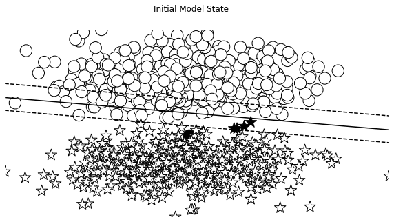
Let’s put everything we learned so far to tackle a classic problem, the toy problem: classifying 2D points into one of two classes. We will be creating a decision boundry, otherwise known as a hyperplane.
Constructing Toy Data
We need to create a simple dataset that can be easily split by a line when seen graphically.
LEFT_CENTER = (3, 3)
RIGHT_CENTER = (3, -2)

def createData(batch_size, left_center=LEFT_CENTER, right_center=RIGHT_CENTER):
    x_data = []
    y_targets = np.zeros(batch_size)
    for batch_i in range(batch_size):
        if np.random.random() > 0.5:
            x_data.append(np.random.normal(loc=left_center))
        else:
            x_data.append(np.random.normal(loc=right_center))
            y_targets[batch_i] = 1
    return torch.tensor(x_data, dtype=torch.float32), torch.tensor(y_targets, dtype=torch.float32)
Choosing a Model
The model being used will be the custom one that we created in the beginning of the lesson, the perceptron, as it is very flexible and allows for any size of input. We shall assign numbers to each of the classes, 1 and 0, which will stay the same throughout the whole process. Keep in mind that the Perceptron that we made is taking advantage of the Sigmoid.
Converting the Probabilities to Discrete Classes
Since this is a binary classification problem, we need to be able to create a decision boundry. Since we have already defined the values for each class, 1 and 0, we can place the hyperplane smack dab in the middle at 0.5. In a real world scenario however, one should tune the value of the hyperplane to the data.
Choosing a Loss Function
As previously mention, being a binary classification model, a BCE Loss Function makes the most sense so that is what we will be using.
Choosing an Optimizer
The optimizer in a model is what updates the model’s weights during training. The learning rate is how much the weights will change by each run. A high learning rate will have issues converging on accurate weights.
We will be using the Adagrad (Adam) optimzer which is an adaptive optimizer meaning it updates with new information.
import numpy as np

lr = 0.01
input_dim = 2

batch_size = 1000
n_epochs = 12
n_batches = 5

seed = 1337

torch.manual_seed(seed)
torch.cuda.manual_seed_all(seed)
np.random.seed(seed)

perceptron = Perceptron(input_dim=input_dim)
optimizer = torch.optim.Adam(params=perceptron.parameters(), lr=lr)
bce_loss = nn.BCELoss()
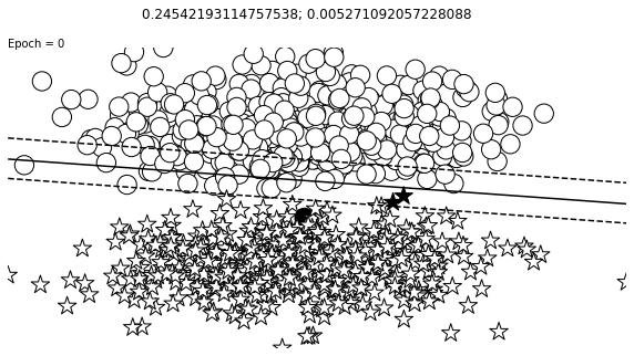
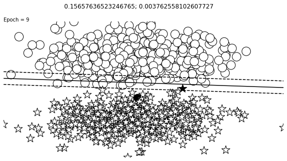
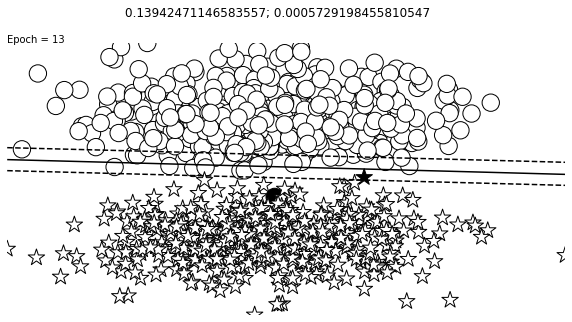
Putting It Together: Gradient-Based Supervised Learning
Learning starts with seeing how far off the model predictions are from the target and the gradient tells how much the parameters should change by. Lets split the training data into batches so that every gradient step uses one batch.
After a certain number of batches, we will have completed one epoch, or a complete training iteration.
def visualize_results(perceptron, x_data, y_truth, n_samples=1000, ax=None, epoch=None,
                      title='', levels=[0.3, 0.4, 0.5], linestyles=['--', '-', '--']):
    y_pred = perceptron(x_data)
    y_pred = (y_pred > 0.5).long().data.numpy().astype(np.int32)

    x_data = x_data.data.numpy()
    y_truth = y_truth.data.numpy().astype(np.int32)

    n_classes = 2

    all_x = [[] for _ in range(n_classes)]
    all_colors = [[] for _ in range(n_classes)]

    colors = ['black', 'white']
    markers = ['o', '*']

    for x_i, y_pred_i, y_true_i in zip(x_data, y_pred, y_truth):
        all_x[y_true_i].append(x_i)
        if y_pred_i == y_true_i:
            all_colors[y_true_i].append("white")
        else:
            all_colors[y_true_i].append("black")
        #all_colors[y_true_i].append(colors[y_pred_i])

    all_x = [np.stack(x_list) for x_list in all_x]

    if ax is None:
        _, ax = plt.subplots(1, 1, figsize=(10,10))

    for x_list, color_list, marker in zip(all_x, all_colors, markers):
        ax.scatter(x_list[:, 0], x_list[:, 1], edgecolor="black", marker=marker, facecolor=color_list, s=300)


    xlim = (min([x_list[:,0].min() for x_list in all_x]),
            max([x_list[:,0].max() for x_list in all_x]))

    ylim = (min([x_list[:,1].min() for x_list in all_x]),
            max([x_list[:,1].max() for x_list in all_x]))

    # hyperplane

    xx = np.linspace(xlim[0], xlim[1], 30)
    yy = np.linspace(ylim[0], ylim[1], 30)
    YY, XX = np.meshgrid(yy, xx)
    xy = np.vstack([XX.ravel(), YY.ravel()]).T

    Z = perceptron(torch.tensor(xy, dtype=torch.float32)).detach().numpy().reshape(XX.shape)
    ax.contour(XX, YY, Z, colors='k', levels=levels, linestyles=linestyles)

    plt.suptitle(title)

    if epoch is not None:
        plt.text(xlim[0], ylim[1], "Epoch = {}".format(str(epoch)))
losses = []
x_data_static, y_truth_static = createData(batch_size)
fig, ax = plt.subplots(1, 1, figsize=(10,5))
visualize_results(perceptron, x_data_static, y_truth_static, ax=ax, title='Initial Model State')
plt.axis('off')
#plt.savefig('initial.png')
change = 1.0
last = 10.0
epsilon = 1e-3
epoch = 0
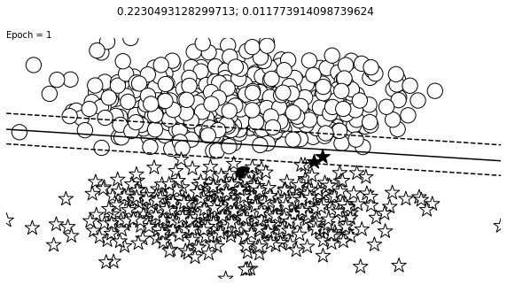
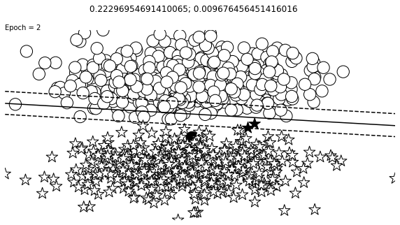
while change > epsilon or epoch < n_epochs or last > 0.3:
#for epoch in range(n_epochs):
for _ in range(n_batches):
optimizer.zero_grad()
x_data, y_target = createData(batch_size)
y_pred = perceptron(x_data).squeeze()
loss = bce_loss(y_pred, y_target)
loss.backward()
optimizer.step()
loss_value = loss.item()
losses.append(loss_value)
change = abs(last - loss_value)
last = loss_value
fig, ax = plt.subplots(1, 1, figsize=(10,5))
visualize_results(perceptron, x_data_static, y_truth_static, ax=ax, epoch=epoch,
title=f"{loss_value}; {change}")
plt.axis('off')
epoch += 1


Auxiliary Training Concepts
Evaluation Metrics
We will be measuring the accuracy of the model in this case but there are other ways to evaluate the success/performance of a model.
Splitting the Dataset
The goal of a model is to generalize well to the true distribution of data. To accomplish this, it is standard practice to split a dataset into three partitions. The training, validation, and test datasets are partitioned into three separate sets separated by class labels.
A common split percentage is to reserve 70% for training, 15% for validation, and 15% for testing. The k-fold process involves splitting the entire dataset into k equally sized “folds” so that each fold can be an evaluation fold and will generate k accuracy values.
Knowing When to Stop Training
The example earlier trained the model for a fixed number of epochs. One key function of correctly measuring model performance is to use that to decide when to stop early by a given patience value.
Early stopping works by keeping track of the performance on the validation dataset until the performance continues to not improve by the patience value. Once below the value, the training is then terminated.
Finding the Right Hyperparameters
Choosing the right loss function, optimizer, learning rate, layer size, patience, and regularization decisions can affect everything about the model and its performance.
Regularization
Recall that most machine learning algorithms are optimizing the loss function to find the most likely values of the parameters (or “the model”) that explains the observations (i.e., produces the least amount of loss).
However, there may sometimes be more than one solution, our job is to find the best one. By appealing to Occam’s razor, we intuit that the simpler explanation is better than the complex one. This smoothness constraint in machine learning is called L2 regularization. another popular regularization is L1 regularization. L1 is usually used to encourage sparser solutions; in other words, where most of the model parameter values are close to zero.
Enjoy Reading This Article?
Here are some more articles you might like to read next: